Naive Bayes Classifiers

7 min readJan 10, 2021

In this blog, we will cover Naive Bayes Classifier and also compare it with other commonly used algorithms.

Naive Bayes classifiers are a collection of classification algorithms based on Bayes’ Theorem. It is not a single algorithm but a family of algorithms where all of them share a common principle, i.e. every pair of features being classified is independent of each other. It’s not possible for a real world data often but still we assume it as it works well and that’s why it is known as naive. It also assumes that each feature makes an equal contribution to the outcome, i.e. each feature is given the same weight.

Bayes Theorem-

Bayes’ Theorem finds the probability of an event occurring given the probability of another event that has already occurred. Bayes’ theorem is stated mathematically as the following equation:

where A and B are events and P(B) ? 0.

Basically, we are trying to find probability of event A, given the event B is true. Event B is also termed as evidence.
P(A) is the priori of A (the prior probability, i.e. Probability of event before evidence is seen). The evidence is an attribute value of an unknown instance(here, it is event B). A is also referred as hypothesis.
P(A|B) is a posteriori probability of B, i.e. probability of event after evidence is seen.
P(B|A) is known as likelihood.

Now, with regards to our dataset, we can apply Bayes’ theorem in following way:

where, y is class variable and X is a dependent feature vector (of size n) where:

Now, its time to put a naive assumption to the Bayes’ theorem, which is, independence among the features. So now, we split evidence into the independent parts.

Now, if any two events A and B are independent, then,

P(A,B) = P(A)P(B)
Final result is —

Now, as the denominator remains constant for a given input, we can remove that term:

Now, we need to create a classifier model. For this, we find the probability of given set of inputs for all possible values of the class variable y and pick up the output with maximum probability. This can be expressed mathematically as:

Using the above function, we can obtain the class, given the predictors.

Types of Naive Bayes Classifier-

The different naive Bayes classifiers differ mainly by the assumptions they make regarding the distribution of P(xi | y).

Multinomial Naive Bayes:

This is mostly used for document classification problem, i.e. whether a document belongs to the category of sports, politics, technology etc. The features/predictors used by the classifier are the frequency of the words present in the document.

In this case distribution of probabilities for each event bases on the formula:

Ny is the total number of features of the event y , Nyi — count of each feature , n — the number of features and α is a smoothing Laplace parameter to discard the influence of words absent in the vocabulary.

from sklearn.naive_bayes import MultinomialNB

Bernoulli Naive Bayes:

This is similar to the multinomial naive bayes but the predictors are boolean variables. The parameters that we use to predict the class variable take up only values yes or no, for example if a word occurs in the text or not.

from sklearn.naive_bayes import BernoulliNB

If handed any other kind of data than binary, a BernoulliNB instance may binarize its input (depending on the binarize parameter).

Gaussian Naive Bayes classifier-

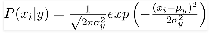
If our data is continuous, we assume that these values are sampled from a gaussian distribution and use Gaussian Naive Bayes Classifier.

Since the way the values are present in the dataset changes, the formula for conditional probability changes to,

from sklearn.naive_bayes import GaussianNB

Another common technique for handling continuous values is to use binning to discretize the feature values, to obtain a new set of Bernoulli-distributed features; some literature in fact suggests that this is necessary to apply naive Bayes, but it is not, and the discretization may throw away discriminative information.

Sklearn also has other models such as-

Complement Naive Bayes-

CNB is an adaptation of the standard multinomial naive Bayes (MNB) algorithm that is particularly suited for imbalanced data sets. Specifically, CNB uses statistics from the complement of each class to compute the model’s weights. The inventors of CNB show empirically that the parameter estimates for CNB are more stable than those for MNB. Further, CNB regularly outperforms MNB (often by a considerable margin) on text classification tasks.

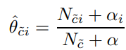
Nc — total number of words in the opposite class , Nci — repetitions of a word in the opposite class . We also use the same smoothing parameters. After the calculation of basic values we start working with the real parameters:

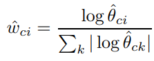
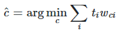
It is the weight for each word in the message of k words. The final decision is calculated by the formula:

from sklearn.naive_bayes import ComplementNB

Categorical Naive Bayes-

The categorical Naive Bayes classifier is suitable for classification with discrete features that are categorically distributed. The categories of each feature are drawn from a categorical distribution.

from sklearn.naive_bayes import CategoricalNB

Applications-

Naive Bayes algorithms are mostly used in sentiment analysis, spam filtering, recommendation systems etc. Means, it is mainly used for text classification tasks as they have higher success rates than other machine learning algorithms. They are fast and easy to implement and hence can we used for real time prediction. But their biggest disadvantage is that the requirement of predictors to be independent. In most of the real life cases, the predictors are dependent, this hinders the performance of the classifier.

Advantages-

It is fast, and easy to understand
It is not prone to overfitting
It only requires a small number of training data to estimate the parameters necessary for classification.
It is faster than Random forest, since it can adapt to changing data pretty quickly. If the assumptions of Naive Bayes hold true, then it is much faster than logistic regression as well.
It perform well in case of categorical input variables compared to numerical variable(s).
Can handle missing values

Disadvantages-

It’s assumptions may not always hold true.
If you have huge feature list, the model may not give you accuracy, because the likelihood would be distributed and may not follow the Gaussian or other distribution.

Tips to improve the power of Naive Bayes Model-

If continuous features do not have normal distribution, we should use transformation or different methods to convert it in normal distribution.
If test data set has zero frequency issue, apply smoothing techniques “Laplace Correction” to predict the class of test data set. If categorical variable has a category (in test data set), which was not observed in training data set, then model will assign a 0 (zero) probability and will be unable to make a prediction. This is often known as “Zero Frequency”.
Remove correlated features
The calculation of the likelihood of different class values involves multiplying a lot of small numbers together. This can lead to an underflow of numerical precision. As such it is good practice to use a log transform of the probabilities to avoid this underflow.
To improve accuracy of Naive Bayes model, data preprocessing and feature selection have more effect than tuning hyperparameters.

Naive Bayes vs other classifiers-

Logistic Regression-

Naive Bayes is a generative model and Logistic regression is a discriminative model. Both Naive Bayes and Logistic regression are linear classifiers and in short Naive Bayes has a higher bias but lower variance compared to logistic regression. On small datasets you’d might want to try out naive Bayes, but as your training set size grows, you likely get better results with logistic regression. Naive Bayes may outperform Logistic Regression if it’s assumptions is fulfilled. Also, Naive Bayes requires good feature engineering to give good results.

KNN-

Naive Bayes is an eager learning classifier and it is much faster than K-NN. Thus, it could be used for prediction in real time. Also, Naive Bayes is a linear classifier so it may give good result only when decision boundary is linear. Otherwise KNN has better chances to give more accuracy for complex decision boundaries.

Decision Trees-

Decision trees require very less or no feature engineering while Naive Bayes require good feature engineering. Decision trees have lower bias but higher variance than naive bayes generally. But there high variance problem can be solved by using random forest. Also, decision trees are much more complex than naive bayes. But again, it may outperform Decision trees if there is low data.

SVM-

Naive bayes may only outperform SVM when there is less data available. But naive bayes classifier is much faster than SVM. There’s also a model NBSVM which combines both models and give a outstanding result when given good amount of data. It actually gives log count of naive bayes as features to SVM. It does not outperform neuarl net but still gives outstanding result.

Neural network-

Again, Naive Bayes may outperform any neural network only when data is less.